Users of Microsoft Excel spreadsheets may need to change rows and columns for a variety of reasons. Moving rows and columns in Excel is as simple as using cut and paste or the shortcut keys Ctrl + X and Ctrl + V, which you may already be familiar with from working in Excel, MS Word, or other programs.
Understanding how to shift rows and columns in Excel is just as crucial as understanding how to copy and paste. This is something you will have to do a lot when you are working with Excel.
Continue reading to learn how to shift columns and rows in Excel using copy/paste and another method shown with screenshots.
How to Move Columns in Excel
There are basically three different ways to move columns in Excel. These ways are:
- Moving Column by Mouse Drag
- Moving Column using Short Keys
- Moving Column using Mouse Right Click
Choose the method that is easiest for you to understand. To move columns in Excel, being familiar with one step is sufficient.
Moving Column by Mouse Drag
Kindly follow these instructions to move a column to the location of your choice using the mouse.
Step 1: Select a column you want to move (we took Column D as an example).
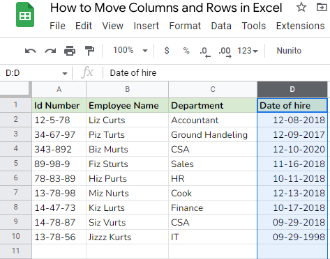
Step 2: Bring the mouse pointer over the edge of the cell in the selected column to transform it into a move pointer. The image that follows shows a border with a move pointer:

Step 3: You can move the column by dragging the move pointer to where you want it to go. For example, we want to shift column D to column C, so we will drag column D and keep it in column C.
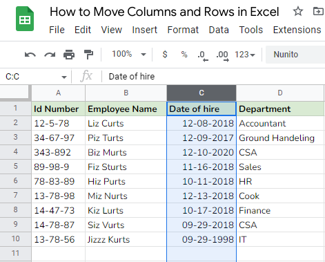
Following this way, the column can be easily moved to your desired location.
Note: This procedure cuts the column and pastes it into the new position. If you want to copy the column to the new spot while keeping the column you already have, just press the Ctrl key before dragging the column to the new place.
Moving Column Using Short Keys
To move a column by short key, follow this:
- Step 1: Choose the column you want to shift, as explained in the previous example.
- Step 2: If you are using Windows, press Ctrl+X. If you are on the Mac operating system, use Command + X.
- Step 3: Choose the column letter where you want to paste it. In our example, we chose C. (We want column D to be shifted into column C.)
- Step 4: Now, on Windows, press Ctrl + V, and on Mac, Command + V.
Note: If you wish to copy the material rather than cut/paste it, replace Ctrl + X with Ctrl + C or Command + C in step 2.
Moving Column using Mouse Right Click
Step 1: Choose a heading column that you want to shift, just like we did in the previous two methods.
Step 2: Press Ctrl + X on Windows or Command + X on Mac OS from the keyboard. This should make the selected borders dotted, as shown in the picture below.
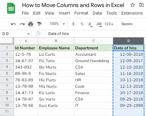
Step 3: The column has been selected; now single on the column you want to paste the selected column on, and press Ctrl + V (Windows) or Command + V (Mac).

Similar to how we shifted Column D to Column C, you will be able to copy and paste the chosen column in the desired location.
Again, if you wish to copy the material rather than cut/paste it, replace Ctrl + X with Ctrl + C or Command + C in step 2.
Note: When you move columns, Excel copies the text and any formulas. This causes hidden cells, values, and cell formats to move.
Cell references are not modified, though. The column references must be manually adjusted.
For instance, if other cells, such as those in column B, are referencing the D cells, they will continue to reference even after the material has been copied to column C. This could result in a #REF! the problem, so be careful.
How to Move Multiple Columns in Excel
You now understand how to move a column in Excel. Yet, do you know how to shift multiple columns continuously?
Suppose we have a dataset in which we wish to move column A and column B before column D.
Now, follow these instructions to gain clarity.
Step 1: Select column A by clicking on the header. Again, press the Shift key and select the header for column B. Do not leave the Shift key until you click on Column B.
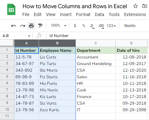
Step 2: Move the mouse over Column B\’s border until the plus symbol appears.
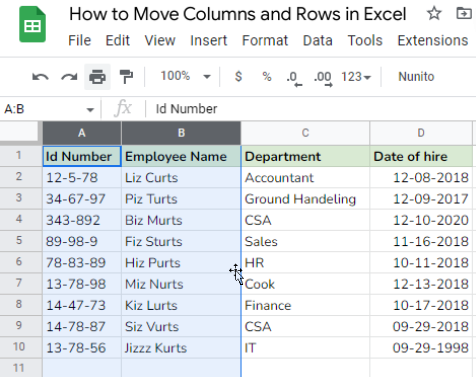
Step 3: Hold and drag the selected columns and drop them before column D, the result will display something like this.
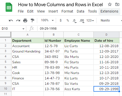
Note: Remember that this hack only works with contiguous columns or rows. It cannot be used to transfer non-contiguous Excel rows and columns.
How to Move Rows in Excel
We will go through the two possible ways to move the rows in excel.
Moving Rows by Mouse Drag
Relocating one or more rows follows almost the same approach as moving columns. Follow these instructions in order to relocate one or more rows. We will shift rows 4 and 5 to positions 7 and 8.
Step 1: Pick a row by selecting the number located on the left side. If you wish to choose multiple rows, click the Shift key and continue selecting rows. Multiple selections should look something like this:
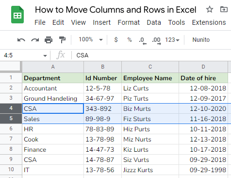
Step 2: Bring the cursor into view by moving the mouse over the thick blue border.
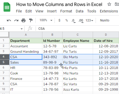
Step 3: Move the mouse down the page and stop at row 7 (for our demo). As required, you will move it to the destination row.
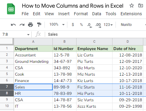
As said earlier, we moved rows 4 and 5 to destinations 7 and 8.
Moving Rows Using Short Keys
You may also move rows using keyboard shortcuts.
- Step 1: Choose the rows you wish to move, as shown in the example above. I selected rows 4 and 5.
- Step 2: Press Ctrl + X for Windows or Command + X for Mac users.
- Step 3: Go to the first cell of the 7th row, i.e., A7 (in our demo), and press Ctrl + V for Windows or Command + V for Mac users.
Following this, you will be able to move the row to your desired position.
Bonus: How to convert data from rows to columns (or vice versa) in Excel
Excel has you covered if you started entering data in a vertical order (columns) and then decided that a horizontal order (rows) would be better. See the picture below for the example:
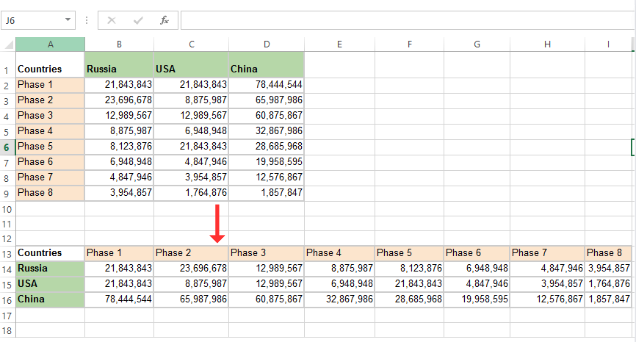
Do the following steps to turn rows into columns:
Step 1: Select the original data you want to change. To quickly select the entire table, or all of the data-containing cells in a spreadsheet, press Ctrl + Home followed by Ctrl + Shift + End.
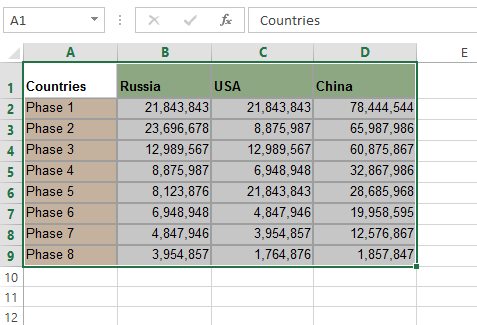
Step 2: Select Copy from the context menu or press Ctrl + C on the keyboard to copy the selected cells.
Step 3: Select the first cell where you want to paste the modified data. Like in the picture below, we chose A13 to paste the modified data.
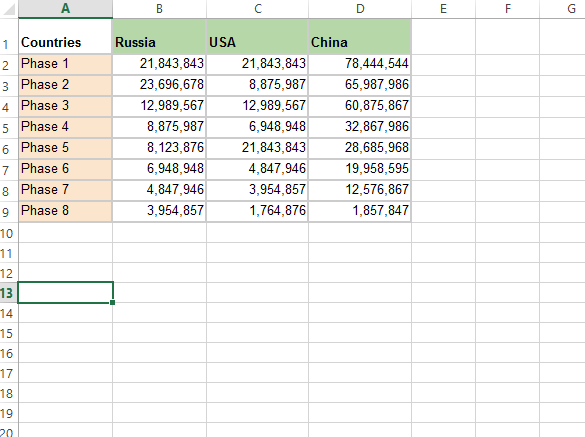
Note: Choose a cell outside of the range where your original data is so that the areas where you copy and paste do not overlap. For example, our original table has four columns and nine rows; the converted table will have nine columns and four rows.
Step 4: Click the right mouse button on the destination cell, pick Paste Special from the context menu, and then select Transpose.
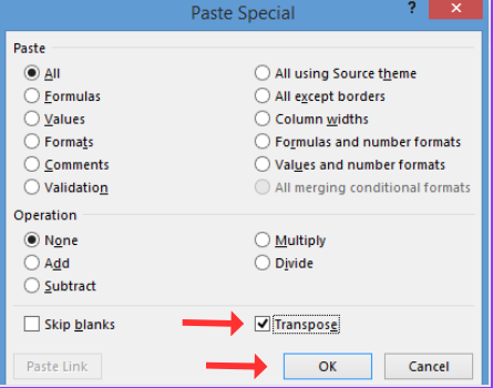
Note: If your source data has formulas, make sure to use relative and absolute references correctly, depending on whether you want to change the formulas or keep them locked to certain cells.
Conclusion
Using Shift, CTRL, and the Insert method, we learned in this post how to quickly shift columns and rows in Excel.
At times, working on an Excel spreadsheet can be somewhat difficult. But if you know how to use these simple features, you may be able to make your spreadsheets more useful and less time-consuming.
