When you start scrolling through a large Excel spreadsheet, it can be hard to remember what kind of information is in the columns and rows. During this time, your job will be easier if you freeze the top columns where your headlines are. Using the Freeze Panes feature and a few other Excel tools, this is an easy and doable task.
This guide explains how to freeze cells in Excel so that they stay visible while you move to another part of the worksheet. Here are the detailed steps for freezing the first column and one or more columns in Excel at the same time.
How to Freeze First Columns in Excel
If you want to freeze the initial columns in Excel, you just need to follow these simple instructions.
Step 1: Click the View tab, which is found at the very top of Excel.
Step 2: Choose Freeze Panes > Freeze First Column from the menu.
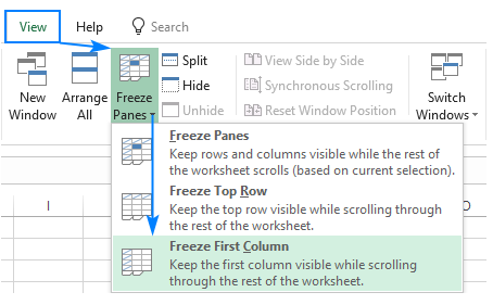
This will freeze the first column from moving. This column should be visible for that worksheet even as you scroll to the right, regardless of where you are in the document.
Note 1: To freeze the top row, you can also tap the Freeze Panes menu and click Freeze Top Row.
Note 2: If you freeze the first column, it will only be visible when you move horizontally. If you move down or to the right, the column values shift.
How to Freeze Multiple Columns in Excel
Let’s say we want to freeze the content of columns A and B in the figure below while the rest of the columns move horizontally into view. 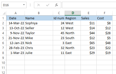
Do the following steps:
Step 1: Choose the column to the right of the last column that you wish to freeze. Here, following the example, we want to freeze the A and B cells, so select the column C or C1 cell.
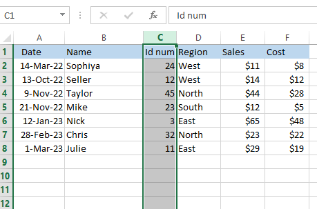
Step 2: Choose View from the ribbon.

Step 3: Search for Freeze Panes group
Step 4: Click the small arrow and select “Freeze Panes,” located in the menu as displayed in the image below.
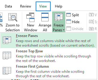
Now, as you scroll horizontally to the right, columns A and B will stay where they are while other columns move.
What if My Freeze Panes Do Not Work?
If the button titled Freeze Panes is disabled (grayed out) on your worksheet, the following are some of the most possible causes for why this is the case:
- You are currently editing a cell, such as by inserting a formula or modifying data. To exit editing mode for a cell, press Enter or Esc.
- Your worksheet has been secured. Please remove the worksheet\’s protection before freezing rows or columns.
However, in addition to freezing panes, Microsoft Excel offers a number of different techniques to lock columns, some of which include the following:
- Split panes rather than freezing it
- Use tables to lock top row in Excel
1. Split Panes rather than Freezing it
In Excel, you may also freeze cells by dividing a worksheet into multiple sections. The distinction is the following:
By Freezing Panes, you can keep certain rows and/or columns in view even as you move around the spreadsheet.
The Splitting Panes command divides the Excel display into two or four scrollable regions. While one area is scrolled, the cells in the remaining area(s) stay constant.
Just following these steps will allow you to split the window in Excel:
Step 1: Pick a cell to the right of the column you wish to split. For example, in the image below, we wish to separate Columns A and B from the remaining columns. Thus, we select Column C.

Step 2: To split the window, select the View tab in the ribbon\’s navigation bar and then click the Split button.
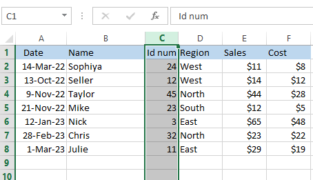
Note: To undo a split, click Split a second time.
2. Use tables to lock top row in Excel
Converting a range in Excel to a table that can perform all of its functions will allow you to make sure that the header row is always displayed at the top of the table, even as you scroll down.
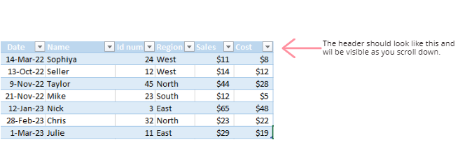
To make a table in Excel as quickly as possible, press the Ctrl + T shortcut.
The Rules of Freezing in Excel
The following is a list of the rules that regulate the process of freezing rows and columns:
- Excel rows and columns cannot be frozen in the middle of the worksheet.
- The freeze panes option can only be used once. Several frozen panes cannot be created in a single spreadsheet.
- During the freezing process, the rows and columns to be locked must be visible. Instead, they will stay hidden after freezing.
Note 1: Use the split option in order to separate a worksheet into two or more sections, each of which will have its own scroll bar. The feature is available in the “window” area of the View tab.
Note 2: Create an Excel table in order to correct the problem of the header row of a large dataset that cannot fit on the screen.
Conclusion
In short, this is how to freeze a column in Excel based on what was said in the post. Because of this, we won’t really have to continually scroll up to the row headers in order to figure out what a particular value indicates. This results in significant as well as time savings.
You can reduce the amount of time spent on your task by reading some of our other articles to learn about fundamental Excel techniques that are comparable.
